

CASE STUDIES / PRICING · OCT 2025
Comparing pricing formulas for Argentine LNG supply.
A proposed Bahia Blanca supply contract is added to three modelled buyer portfolios.
3 buyer models
BRENT PRICING GIVES THE HIGHEST SUPPLIER REVENUE IN EACH
Represent three buyer types.
01 · PORTFOLIO
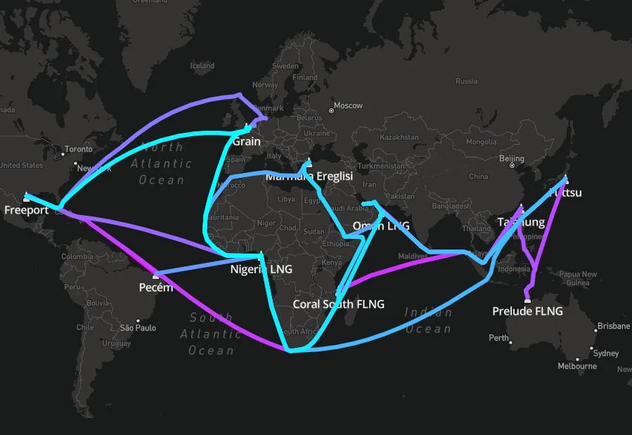
The study models a global major, a Gulf producer and a utility using public information and estimated portfolio sizes. It adds the same Argentine FOB opportunity to each.
GLOBAL MAJOR A · SHELL-SCALE
- 157 FOB purchases across Australia, the Middle East, the US and Africa
- 101 DES sales in Asia, Europe and the Americas · JKM, TTF and Brent
- 22 x 174K vessels · spot access in five markets
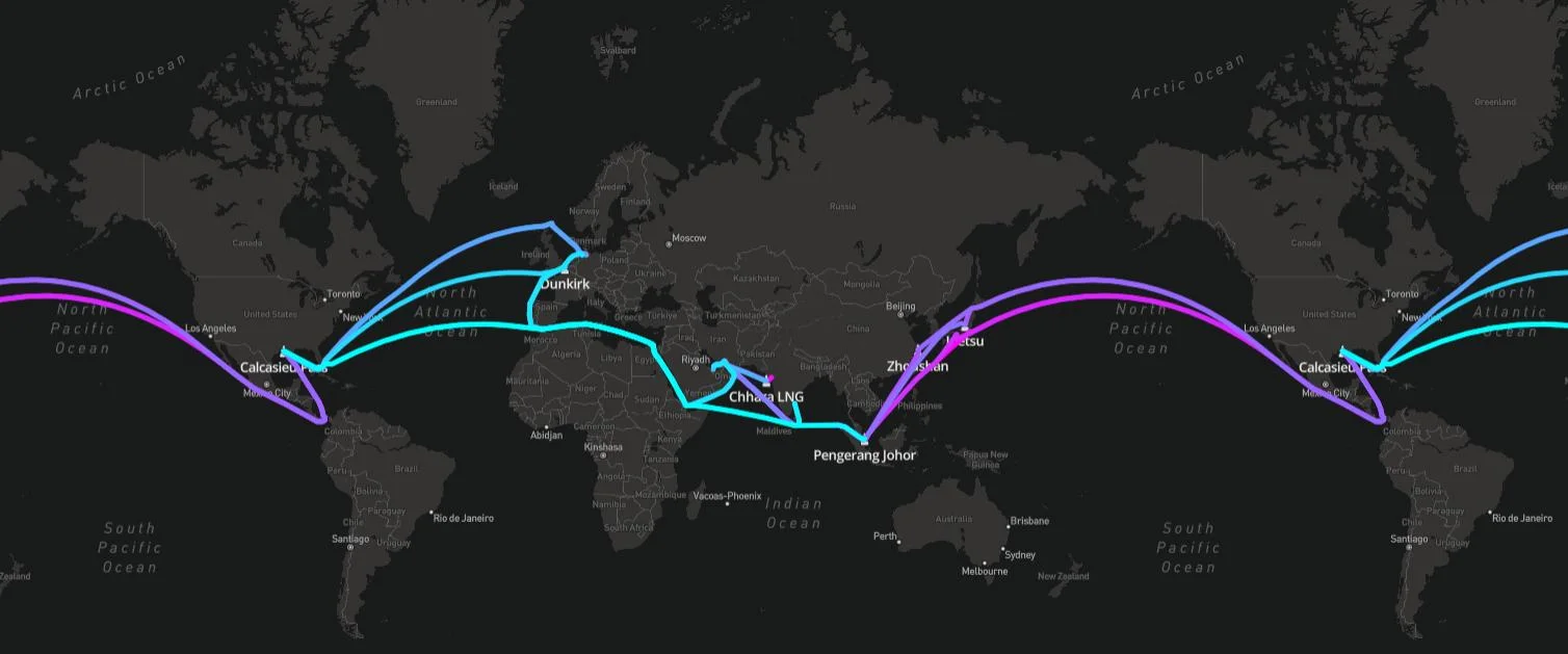
GULF PRODUCER B · ADNOC-SCALE
- 119 Brent-indexed FOB purchases from the Middle East
- 114 DES sales: 82 Asia (JKM), 32 Europe (TTF)
- 20 x 174K vessels · Brent-heavy by construction
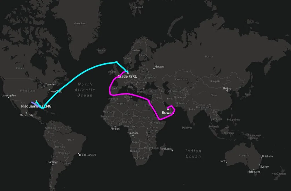
EUROPEAN UTILITY C · ENBW-SCALE
- 33 FOB purchases: 24 US (HH), 9 Middle East (Brent)
- 36 TTF-indexed DES sales into Europe
- 3 x 174K vessels · the smallest modelled portfolio
Modelled buyer portfolios based on public data. Each comparison adds an Argentine FOB supply contract loading at Bahia Blanca.
Vary the formula and discount.
02 · PRICING FORMULAS
The model tests TTF, JKM and Brent indexation with discounts from $0.25 to $5.00/MMBtu. It recalculates the buyer’s schedule for each combination.
Compare total supplier revenue.
03 · SUPPLIER REVENUE
The displayed revenue curves reach their highest values with Brent indexation for each modelled buyer. Compare each formula within the same chart and buyer portfolio. Total revenue also depends on how many cargoes the buyer selects.
Check volume as well as revenue.
04 · REVENUE PER VOYAGE
Revenue per voyage produces a different comparison from total revenue. The global-major model reaches $30.1M per voyage. The discounts associated with the peak totals also differ between buyers.
Compare the discount and volume at each selected result.
05 · SELECTED DISCOUNTS
A larger discount can encourage the buyer to take more cargoes while reducing revenue per unit. The tables report selected scenario results; revenue per voyage and total supplier revenue measure different things.
Selected results from the source scenario table. Buyer profit remains positive at each selected discount.
06 · RESULT
The highest modelled supplier revenue uses Brent indexation for all three buyers.
The buyer portfolios are public-data approximations, not company forecasts or actual procurement plans. Revenue is not profit. Results depend on the assumed portfolio, capacity and pricing curves.
What this comparison shows.
07 · TAKEAWAYS
Vary the formula and discount
The model tests TTF, JKM and Brent indexation with discounts from $0.25 to $5.00/MMBtu. It recalculates the buyer’s schedule for each combination.
Compare the discount and volume at each selected result
A larger discount can encourage the buyer to take more cargoes while reducing revenue per unit. The tables report selected scenario results; revenue per voyage and total supplier revenue measure different things.
Scope of the result
The buyer portfolios are public-data approximations, not company forecasts or actual procurement plans. Revenue is not profit. Results depend on the assumed portfolio, capacity and pricing curves.
How the study was calculated.
08 · CALCULATION
Set up the comparison
The study models a global major, a Gulf producer and a utility using public information and estimated portfolio sizes. It adds the same Argentine FOB opportunity to each.
Calculate the alternatives
The displayed revenue curves reach their highest values with Brent indexation for each modelled buyer. Compare each formula within the same chart and buyer portfolio. Total revenue also depends on how many cargoes the buyer selects.
Review the result
The highest modelled supplier revenue uses Brent indexation for all three buyers.
Modelled results depend on the contracts, prices and operating assumptions used.